Classification
Forecasting
Detecting Hackers Like It's 1999
This tutorial will use the Nexosis API to classify malicious network traffic using prepared network data captured from a Defense Department Network while it was under attack. Given this data, we’ll show how Machine Learning can be used to build a model that will classify network data as malicious or normal based on its characteristics.
Details
Scope: This tutorial will teach more detailed concepts on formatting datasets as well as understanding Classification metrics and understanding the Confusion Matrix.
Time: 20 minutes
Level: Intermediate / 200-level
Prerequisites:
Before starting
It’s important that you understand the following concepts to successfully complete this tutorial.

Obligatory Hackers movie poster - ©1995 United Artists
- Understanding the problem
- Datasets
- Submitting the data to Nexosis
- Building the model
- Results
- Next steps
Understanding the problem
This tutorial will walk through a Data Science competition called the KDD Cup from 1999.
“This is the data set used for The Third International Knowledge Discovery and Data Mining Tools Competition, which was held in conjunction with KDD-99 The Fifth International Conference on Knowledge Discovery and Data Mining.”
The abstract describes the goal of the competition as follows:
“The competition task was to build a network intrusion detector, a predictive model capable of distinguishing between ‘bad’ connections, called intrusions or attacks, and ‘good’ normal connections. This database contains a standard set of data to be audited, which includes a wide variety of intrusions simulated in a military network environment.”
See KDD Cup 1999 Data and Intrustion Detection Learning for more details, including downloads of the prepared data, task description and data dictionary.
The initial program used to create the data for this competition was prepared and managed by MIT Lincoln Labs. They set up an environment that captured raw network traffic (TCP dump data) for a network simulating a typical U.S. Air Force LAN for 9 weeks. While capturing data, they hit it with multiple attacks. They collected about 4 GB of the network data, compressed and then transformed it into almost 5 million connection records and did some post processing to make sure the records contained some information that would be useful to detecting attackers.
Datasets
The data gathered fell into three different categories:
- Basic features of individual TCP connections
- Content features within a connection suggested by domain knowledge.
- Traffic features computed using a two-second time window.
Download Datasets
There are quite a few files made available for the KDD Cup 1999 competition. Here are a list of the ones used for this exercise. All of them won’t be needed in this tutorial, but if you don’t want to use our prepared dataset these allow you to construct your own.
kddcup.data.gz - The full data set, with labels (18M; 743M Uncompressed)
kddcup-data_10_percent.gz - A 10% subset, with labels. (2.1M; 75M Uncompressed)
kddcup.names - A file containing the names of the features, or column headers.
corrected.gz - Corrected Test data, with labels. Can be used to validate the model once it’s built. (1.4M Compressed, 46M Uncompressed)
kddcup-training.csv - Training DataSet prepped and formatted for the Nexosis API using the files above.
kddcup-training-small-balanced.csv - Training DataSet prepped from the full dataset, reduced and balanced for the Nexosis API using the files above (5.4MB).
Here is the data dictionary of each type of features in the dataset:
| feature name | description | type |
|---|---|---|
| duration | length (number of seconds) of the connection | continuous |
| protocol_type | type of the protocol, e.g. tcp, udp, etc. | discrete |
| service | network service on the destination, e.g., http, telnet, etc. | discrete |
| src_bytes | number of data bytes from source to destination | continuous |
| dst_bytes | number of data bytes from destination to source | continuous |
| flag | normal or error status of the connection | discrete |
| land | 1 if connection is from/to the same host/port; 0 otherwise | discrete |
| wrong_fragment | number of ‘wrong’ fragments | continuous |
| urgent | number of urgent packets | continuous |
Table 1: Basic features of individual TCP connections.
| feature name | description | type |
|---|---|---|
| hot | number of ‘hot’ indicators | continuous |
| num_failed_logins | number of failed login attempts | continuous |
| logged_in | 1 if successfully logged in; 0 otherwise | discrete |
| num_compromised | number of ‘compromised’ conditions | continuous |
| root_shell | 1 if root shell is obtained; 0 otherwise | discrete |
| su_attempted | 1 if ‘su root’ command attempted; 0 otherwise | discrete |
| num_root | number of ‘root’ accesses | continuous |
| num_file_creations | number of file creation operations | continuous |
| num_shells | number of shell prompts | continuous |
| num_access_files | number of operations on access control files | continuous |
| num_outbound_cmds | number of outbound commands in an ftp session | continuous |
| is_hot_login | 1 if the login belongs to the ‘hot’ list; 0 otherwise | discrete |
| is_guest_login | 1 if the login is a ‘guest’login; 0 otherwise | discrete |
Table 2: Content features within a connection suggested by domain knowledge.
| feature name | description | type |
|---|---|---|
| count | number of connections to the same host as the current connection in the past two seconds | continuous |
| Note: The following features refer to these same-host connections. | ||
| serror_rate | % of connections that have ‘SYN’ errors | continuous |
| rerror_rate | % of connections that have ‘REJ’ errors | continuous |
| same_srv_rate | % of connections to the same service | continuous |
| diff_srv_rate | % of connections to different services | continuous |
| srv_count | number of connections to the same service as the current connection in the past two seconds | continuous |
| Note: The following features refer to these same-service connections. | ||
| srv_serror_rate | % of connections that have ‘SYN’ errors | continuous |
| srv_rerror_rate | % of connections that have ‘REJ’ errors | continuous |
| srv_diff_host_rate | % of connections to different hosts | continuous |
Table 3: Traffic features computed using a two-second time window.
The above data dictionaries are defined here: Intrustion Detection Learning
The last bit of information required to build a model for classification is labled data. Labeled data is simpley tagging each row of data as normal or assigning it the name of malicious attack it is (e.g. nmap, neptune, warezclient, teardrop, etc). Below are the different labels provided in the datasets from the KDD Cup 1999 dataset. The DataSets contain the specific attack, and each specific attack can be grouped into a more general category.
There are four general attack categories, and one to represent normal traffic:
- Denial of Service (
dos) - User-to-Root (
u2r) - Remote-to-Local (
r2l) - Probe (
probe) - Normal (
normal)
Here are all the specific attack types and what general category they fall under.
| Specific Attack Type | General Attack Category |
|---|---|
| back | dos |
| buffer_overflow | u2r |
| ftp_write | r2l |
| guess_passwd | r2l |
| imap | r2l |
| ipsweep | probe |
| land | dos |
| loadmodule | u2r |
| multihop | r2l |
| neptune | dos |
| nmap | probe |
| perl | u2r |
| phf | r2l |
| pod | dos |
| portsweep | probe |
| rootkit | u2r |
| satan | probe |
| smurf | dos |
| spy | r2l |
| teardrop | dos |
| warezclient | r2l |
| warezmaster | r2l |
| normal | normal (normal traffic, no attack) |
Table 3: Of Attack Types / Classes.
The labeled dataset provided has each row labeled with the specific attack type, but not the General attack cateogry meaning we’ll need to append that column to each row.
Training data
There are many files provided by the competition which can lead to some confusion about which ones to use. There are full datasets with and without labels, 10% dataset with and without labels, as well as test data. Additionally there were some mistakes in the dataset which were subsequently fixed in the original files, which are also available.
Since we’re building a Classification model, we’ll want to use a labeled dataset so we can eliminate any dataset with unlabeled data. Additionaly, we can ignore any test data since that will be used to check the model after it’s built. This leaves the following two files to choose from:
One last catch. The file does not have a CSV header. A CSV header should be added to the top of the csv file. The names of the features, or column headers, are provided in kddcup.names above.
The full dataset is 743MB which is rather large. It’s better to start with a smaller set of data considering more data is more computationally expensive and the accuracy gains deminish after a certain point. We’ll choose the 10% dataset to start out and see how well it performs. 75MB is still potentially larger than it needs to be but we’ll start there, knowing we can futher reduce it later if desired.
To read more about finding the ideal training dataset size, read Data Education: The Value of Data Experimentation blog post.
Prepare Training Data File
Here are the specific steps used to prepare the file to send to the Nexosis API to train a model:
- We already have a prepared training CSV file named
kddcup-training-small-balanced.csvlinked above in the Test data section. You may find it helpful to review the rest of this section. Continue at the Test data section.
OR
If you're using a paid tier, you can download the much larger 10% training file namedkddcup-data_10_percent.gzlinked above from the KDDCUP archives. Proceed through the rest of the steps in this section for a quick tutorial on how to prepare the file for upload. - Decompress the file using a decompression tool, such as 7-ZIP on windows or `gzip` on linux or OS X. The extracted file will be named
kddcup.data_10_percent_corrected. - Create a new file called
kddheader.csvand paste the following in it and save it in the same folder with the uncompressed kddcup data file:duration,protocol_type,service,flag,src_bytes,dst_bytes,land,wrong_fragment,urgent,hot,num_failed_logins,logged_in,num_compromised,root_shell,su_attempted,num_root,num_file_creations,num_shells,num_access_files,num_outbound_cmds,is_host_login,is_guest_login,count,srv_count,serror_rate,srv_serror_rate,rerror_rate,srv_rerror_rate,same_srv_rate,diff_srv_rate,srv_diff_host_rate,dst_host_count,dst_host_srv_count,dst_host_same_srv_rate,dst_host_diff_srv_rate,dst_host_same_src_port_rate,dst_host_srv_diff_host_rate,dst_host_serror_rate,dst_host_srv_serror_rate,dst_host_rerror_rate,dst_host_srv_rerror_rate,typeWARNING: Make sure there is exactly ONE empty line in the
kddheader.csvfile after the header row or you will end up with the first row on the same line as the headers or some blank rows between the header and the data when the files are combined in the next step. - Merge the
kddheader.csvwith thekddcup.data_10_percentfile.
On Windows, from a command prompt, use thecopycommand to merge the files:
On Linux or Mac you can use thecopy kddheader.csv+kddcup.data_10_percent_corrected kddcup-training.csvcatcommand to merge the files:cat kddheader.csv kddcup.data_10_percent_corrected > kddcup-training.csv - You should now have a file named
kddcup-training.csv. Here's a small random selection of data from the file including the csv header:duration,protocol_type,service,flag,src_bytes,dst_bytes,land,wrong_fragment,urgent,hot,num_failed_logins,logged_in,num_compromised,root_shell,su_attempted,num_root,num_file_creations,num_shells,num_access_files,num_outbound_cmds,is_host_login,is_guest_login,count,srv_count,serror_rate,srv_serror_rate,rerror_rate,srv_rerror_rate,same_srv_rate,diff_srv_rate,srv_diff_host_rate,dst_host_count,dst_host_srv_count,dst_host_same_srv_rate,dst_host_diff_srv_rate,dst_host_same_src_port_rate,dst_host_srv_diff_host_rate,dst_host_serror_rate,dst_host_srv_serror_rate,dst_host_rerror_rate,dst_host_srv_rerror_rate,type 0,tcp,http,SF,215,45076,0,0,0,0,0,1,0,0,0,0,0,0,0,0,0,0,1,1,0.00,0.00,0.00,0.00,1.00,0.00,0.00,0,0,0.00,0.00,0.00,0.00,0.00,0.00,0.00,0.00,normal 0,tcp,http,SF,162,4528,0,0,0,0,0,1,0,0,0,0,0,0,0,0,0,0,2,2,0.00,0.00,0.00,0.00,1.00,0.00,0.00,1,1,1.00,0.00,1.00,0.00,0.00,0.00,0.00,0.00,normal 0,tcp,http,SF,236,1228,0,0,0,0,0,1,0,0,0,0,0,0,0,0,0,0,1,1,0.00,0.00,0.00,0.00,1.00,0.00,0.00,2,2,1.00,0.00,0.50,0.00,0.00,0.00,0.00,0.00,normal 21,tcp,ftp,SF,89,345,0,0,0,1,0,1,0,0,0,0,1,0,0,0,0,0,1,1,0.00,0.00,0.00,0.00,1.00,0.00,0.00,255,1,0.00,0.02,0.00,0.00,0.00,0.00,0.00,0.00,rootkit 98,tcp,telnet,SF,621,8356,0,0,1,1,0,1,5,1,0,14,1,0,0,0,0,0,1,1,0.00,0.00,0.00,0.00,1.00,0.00,0.00,255,4,0.02,0.02,0.00,0.00,0.00,0.00,0.00,0.00,rootkit 0,tcp,ftp_data,SF,0,5636,0,0,0,0,0,1,2,0,0,2,0,0,0,0,0,0,1,1,0.00,0.00,0.00,0.00,1.00,0.00,0.00,1,41,1.00,0.00,1.00,0.10,0.00,0.00,0.00,0.00,rootkit 61,tcp,telnet,SF,294,3929,0,0,0,0,0,1,0,1,0,4,1,0,0,0,0,0,1,1,0.00,0.00,0.00,0.00,1.00,0.00,0.00,255,4,0.02,0.02,0.00,0.00,0.00,0.25,0.73,0.25,rootkit 0,tcp,imap4,REJ,0,0,0,0,0,0,0,0,0,0,0,0,0,0,0,0,0,0,239,15,0.00,0.00,1.00,1.00,0.06,0.06,0.00,255,15,0.06,0.08,0.00,0.00,0.00,0.00,1.00,1.00,neptune 0,tcp,imap4,REJ,0,0,0,0,0,0,0,0,0,0,0,0,0,0,0,0,0,0,240,16,0.00,0.00,1.00,1.00,0.07,0.06,0.00,255,16,0.06,0.08,0.00,0.00,0.00,0.00,1.00,1.00,neptune 0,tcp,imap4,REJ,0,0,0,0,0,0,0,0,0,0,0,0,0,0,0,0,0,0,243,17,0.00,0.00,1.00,1.00,0.07,0.06,0.00,255,17,0.07,0.07,0.00,0.00,0.00,0.00,1.00,1.00,neptune 0,icmp,eco_i,SF,8,0,0,0,0,0,0,0,0,0,0,0,0,0,0,0,0,0,1,10,0.00,0.00,0.00,0.00,1.00,0.00,1.00,4,204,1.00,0.00,1.00,0.25,0.00,0.00,0.00,0.00,nmap 0,icmp,eco_i,SF,8,0,0,0,0,0,0,0,0,0,0,0,0,0,0,0,0,0,1,6,0.00,0.00,0.00,0.00,1.00,0.00,1.00,1,205,1.00,0.00,1.00,0.25,0.00,0.00,0.00,0.00,nmap 0,icmp,eco_i,SF,8,0,0,0,0,0,0,0,0,0,0,0,0,0,0,0,0,0,1,12,0.00,0.00,0.00,0.00,1.00,0.00,1.00,2,206,1.00,0.00,1.00,0.25,0.00,0.00,0.00,0.00,nmap 0,tcp,other,REJ,0,0,0,0,0,0,0,0,0,0,0,0,0,0,0,0,0,0,510,1,0.22,0.00,0.78,1.00,0.00,1.00,0.00,255,1,0.00,1.00,0.00,0.00,0.25,0.00,0.75,1.00,satan 0,tcp,other,REJ,0,0,0,0,0,0,0,0,0,0,0,0,0,0,0,0,0,0,510,1,0.22,0.00,0.78,1.00,0.00,1.00,0.00,255,1,0.00,1.00,0.00,0.00,0.25,0.00,0.75,1.00,satan 0,tcp,other,REJ,0,0,0,0,0,0,0,0,0,0,0,0,0,0,0,0,0,0,510,1,0.22,0.00,0.78,1.00,0.00,1.00,0.00,255,1,0.00,1.00,0.00,0.00,0.25,0.00,0.75,1.00,satan - (Optional) - In the Original CSV, every line in the CSV is terminated with a period. Because of that, all the items in the
typecolumn will contain a period (e.g.noraml.,satan.,buffer_overflow., etc.) If you are on linux or mac, or if you have unix tools installed on windows (i.e. gitbash, cygwin, etc.) you can quickly clean this up using thesedcommand with a regular expression, like so:sed -i -e 's/\.$//' kddcup-training.csv - IMPORTANT CRITICAL FINAL STEP BEFORE SUBMITTING TO NEXOSIS API: Validate the CSV file.
Notice the odd square on line494023below?
 This needs removed or the import will encounter an error due to an illegal character in the file. An easy way to fix this in bash is with the
 headcommand, which removes the last line:head -n -1 kddcup-training.csv > kddcup-training.tmp ; mv kddcup-training.tmp kddcup-training.csv
If there are any illeagal characters, jagged rows, unpaired quotations around strings, extra commas, etc. the Import will fail. The Nexosis API will attempt to provide details in Response body as to where the error was encountered. In this case, the file we downloaded has an illegal byte at the end of the file. By opening reviewing the file in Visual Studio Code, Notepad++, or another text editor, it can help identify issues. Excel can help validate there are no jagged rows, but it can also mask other issues as well.
Avoid using
Alternativly, if the file is not too large you can use Notepad++, Visual Studio Code, Atom, etc. to review and make manual tweaks to the file.notepad.exeto review CSV files unless the file is very small - small in both number of rows as well as the length of each line. Notepad has proven time and again to be increadibly unreliable in many ways.
For some common tools used for data munging, read 5 Text Transforming Techniques for Total Techies.
Test data
Now that the training dataset has been prepared, an additional test dataset can used to further validate if the model is working as it should. A test dataset must also be labeled so the predicted value and the actual value can be compared. For the competition, teams are given an unlabeled test dataset to perform predictions on and the judges would then compare those predictions to the actuals they kept hidden (just like Kaggle competitions work). This prevents teams from cheating by having the answer key. by biasing the model towards the the test set used for judging. Since the competition is over, a labeled test set was released so anyone can validate their test set against the answer key.
The corrected.gz file listed above contains labeled test dataset. After the model is built, we can use this dataset to measure our model performance against data it’s never seen before - so you can proove there’s no tricks up our sleeves. For now, there’s nothing to do with this file other than save it later to calculate metrics to get a more realistic sense of the model’s accuracy.
Submitting the data to Nexosis
Since the dataset is larger than the maximum POST size allowed by the API, the file will need to be uploaded in batches (1MB at a time), or hosted at a URL.
In this tutorial, Digital Ocean Spaces is used for file storage to host the training dataset file. Nexosis API also supports files stored in AWS S3, Azure Blob, or any URL that contains a path to a CSV file or properly formatted JSON file.
For more information on Importing JSON and CSV Files, see the documentation on Importing Data in the documentation to import data from other sources.
- To create a Space in Digital Ocean, create and account and login. Click
Spaceslink in the nav bar at the top.
-
Once you are in the Spaces area, click the green
Createbutton in the uppper right. Choose type a Space Name, datacenter region, and file listing permission: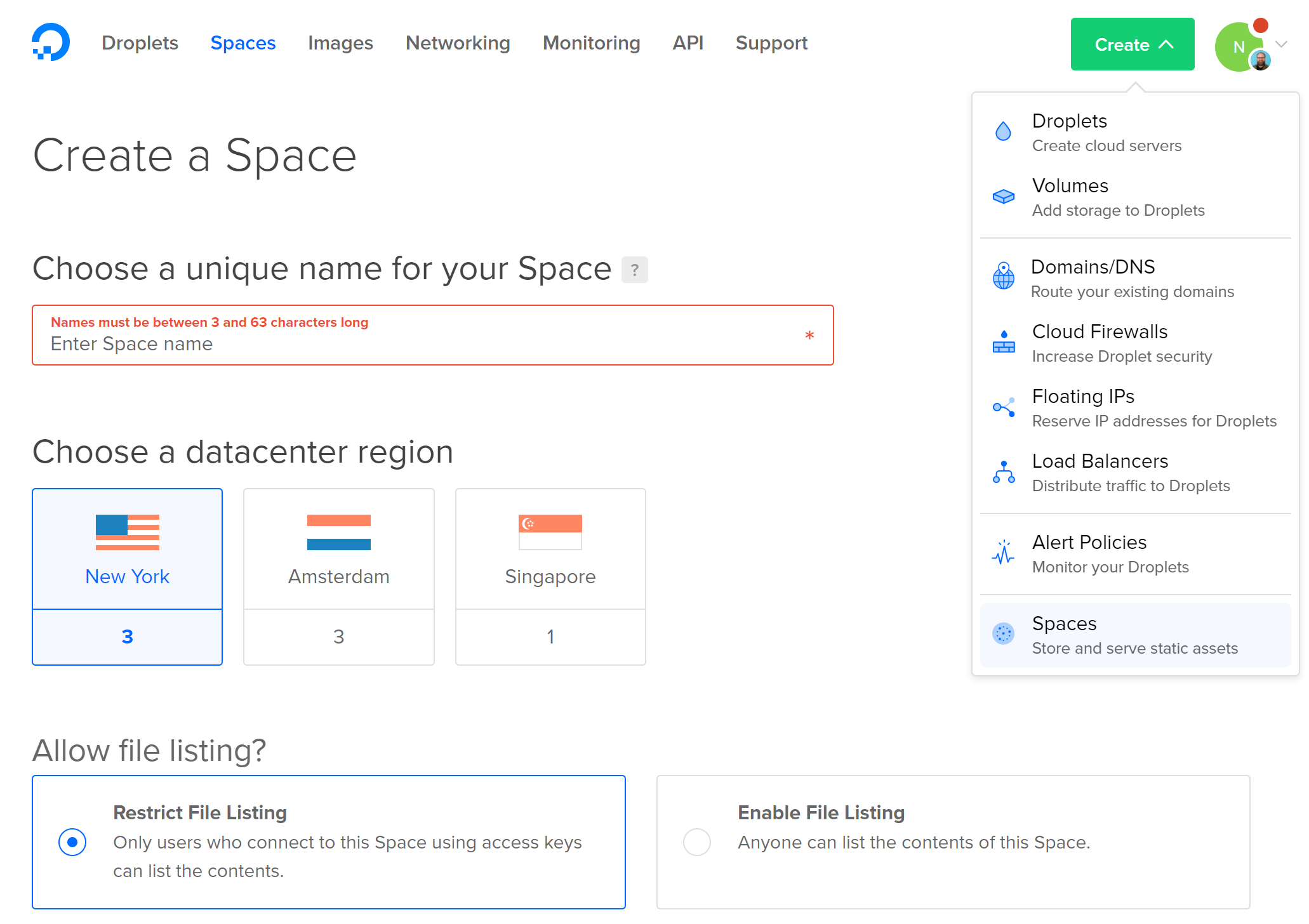
-
Once the space is created, click the blue
Upload Filesbutton. Upload thekddcup-training.csvfile. Since there’s nothing sensitive in this file, make sure to make itPublically Readable.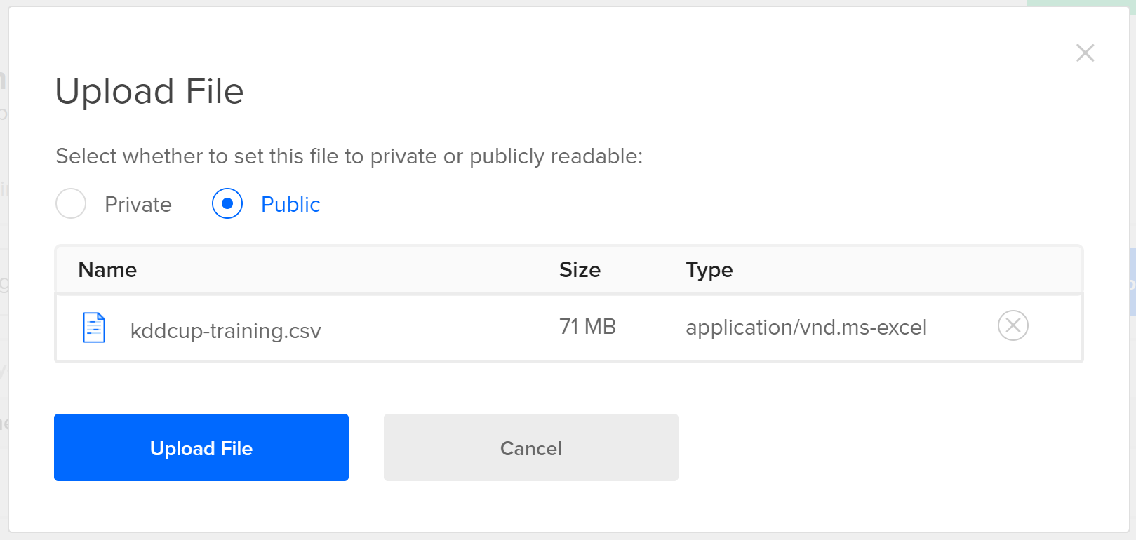
-
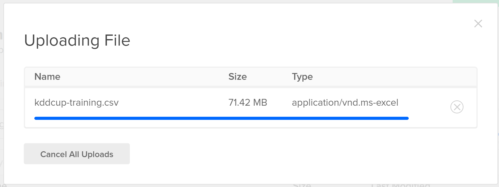
Wait for the file to finish uploading.
-
Once the upload has completed, hover over the file and wait for the pop-up. Click the
Copy URLbutton to get a public link to the training file.
-
The URL should look something like this:
https://jm0nty-public.nyc3.digitaloceanspaces.com/kddcup-training.csv
If using the smaller prepared dataset, the URL should look like this:
https://jm0nty-public.nyc3.digitaloceanspaces.com/kddcup-training-small-balanced.csv
Now that the the large training dataset is in a place where it can be retrieved, the Nexosis API needs instructions to import it. To import a file from Digital Ocean Spaces, we need to send an HTTP POST request to https://ml.nexosis.com/v1/imports/Url. In the HTTP request body, the following JSON will tell the Nexosis API what URL to retrieve the data from and the name to give the dataset:
{
    "dataSetName": "kddcup-training",
    "url": "https://jm0nty-public.nyc3.digitaloceanspaces.com/kddcup-training.csv"
}
OR for the smaller file:
{
    "dataSetName": "kddcup-training",
    "url": "https://jm0nty-public.nyc3.digitaloceanspaces.com/kddcup-training-small-balanced.csv"
}
Here are the steps to accomplish this using the JSON above:
- Open Postman, in the Nexosis Postman Collection, expand the Imports and select
Import from URL.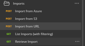
The HTTP Verb is set toPOST, and the URL tohttps://ml.nexosis.com/v1/imports/Url. TheAccept,Content-Type, andapi-keyheaders should be set as follows:
For information on finding your API key, read this support article.
- Click on the request
Bodytab in Postman and include theJSONfrom above:
- Click
Sendin Postman and receive something similar to the following HTTP response from the API: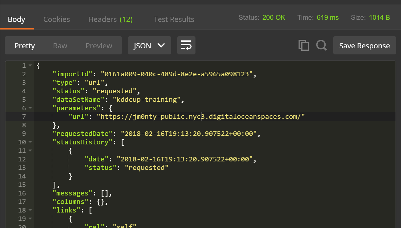
Important: Copy the
importIdout of the response body as you will need this in the next step to check on the Import progress. - In a new Postman request, send a
GETrequest tohttps://ml.nexosis.com/v1/imports/{importId}and replace{importid}with the ID saved from the previous step.
- Keep checking back every few minutes until
"status": "completed"is reported in thestatusHistoryarray in the JSON response....data elided... "statusHistory": [ { "date": "2018-02-16T22:33:56.297532+00:00", "status": "requested" }, { "date": "2018-02-16T22:33:56.8138766+00:00", "status": "started" }, { "date": "2018-02-16T22:42:56.3124271+00:00", "status": "completed" } ], ...data elided...
Now that the training data has been submitted to the Nexosis API, experimentation with building a model can commence.
Building the model
- From the Nexosis API Collections, open the Sessions folder and click
POST /sessions/model.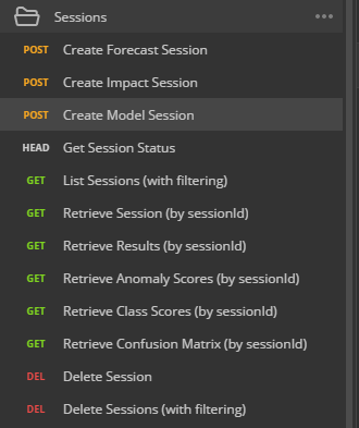
If you don’t have the Nexosis API collections, you can simply selectPOSTfrom the dropdown and typehttps://ml.nexosis.com/v1/sessions/modelin the text bar.
- Click
Bodyand paste the following code. - Note:typewas the column in our dataset that had the network attack type in it (e.g.nmap,neptune,warezclient,teardrop, etc). By settingtypeas the target column, we are telling the Nexosis API to build a model that can predict the attack type based on all the other columns in the dataset, which by default will be used as features.
‘json { "name": "predictAttackType", "dataSourceName": "kddcup-training", "targetColumn": "type", "predictionDomain": "classification" } '
You should have a POST request that looks like this (don’t forget to set theapi-keyheader):

- Click the blue
Sendbutton to the Right of the URL in Postman.

When you inspect to the response body, note the unique session ID and in thestatusHistory, the responsestatusshould sayrequestedorstartedalong with the corresponding timestamp.
{
    // ... column metadata elided
    "sessionId": "0161de6c-d28c-4e0f-84da-a07ed56aa750",
    "type": "model",
    "status": "requested",
    "predictionDomain": "classification",
    "availablePredictionIntervals": [],
    "requestedDate": "2018-02-28T21:58:48.209273+00:00",
    "statusHistory": [
        {
            "date": "2018-02-28T21:58:48.209273+00:00",
            "status": "requested"
        }
    ],
    "extraParameters": {
        "balance": true
    },
    "messages": [],
    "name": "predictAttackType",
    "dataSourceName": "kddcup-training",
    "dataSetName": "kddcup-training",
    "targetColumn": "type",
    "isEstimate": false,
    "links": [
        {
            "rel": "results",
            "href": "https://ml.nexosis.com/v1/sessions/0161de6c-d28c-4e0f-84da-a07ed56aa750/results"
        },
        {
            "rel": "data",
            "href": "https://ml.nexosis.com/v1/data/kddcup-training"
        },
        {
            "rel": "vocabularies",
            "href": "https://ml.nexosis.com/v1/vocabulary?createdFromSessionid=0161de6c-d28c-4e0f-84da-a07ed56aa750"
        }
    ]
}
During a session run, the Nexosis API will automatically split the training data into internal train and test datasets (80% to train, and 20% test cases) when building and tuning its models. Additionally, the Nexosis API will perform cross validation to make sure the model will perform more accurately in practice. It’s not a bad idea to hold back even more test data to validate that the model works with other data it’s never seen before.
Important: Copy your
SessionIDout of the response body as you will need this in the next steps.
Check if session is complete
When the model is finished, you will receive an email with your session ID. You can also check the status of your session with an API call. To do this, you will need the session ID you copied from the previous step.
-
Open the Sessions folder and click
GET /sessions/:sessionId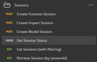
- Click
Paramsand paste the unique session ID forsessionIdValue.Note: Your session ID can be found on the previous Postman tab. For this example, the
sessionIdis0161de6c-d28c-4e0f-84da-a07ed56aa750.
- Click the blue
Sendbutton to the Right of the URL in Postman.

- Scroll to the bottom to check if the status has completed. If the status has completed, your model ID will be provided.
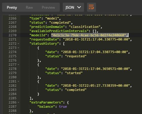
Important: Copy your unique model Id. For this example the
modelIDis4e1c1c3a-79de-4cae-bc56-0d2f4e240668
Results
Now that the model has been created, is it any good? The Session results will contain metrics and the results of the internal test set for review, if desired.
- Open the Sessions folder and click
GET Retrieve Results (by sessionId)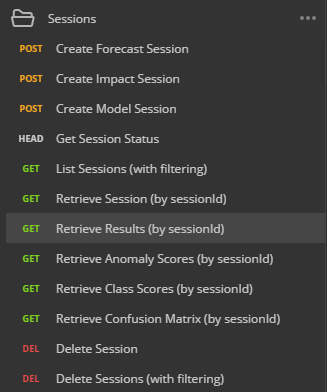
- Click Params and paste the unique session ID for
sessionIdValue.Note: Your session ID can be found on the previous Postman tab. For this example, the
sessionIdis0161de6c-d28c-4e0f-84da-a07ed56aa750.
- Click the blue
Sendbutton to the Right of the URL in Postman.

- The Session Result response body contains both metrics of how accurate the model’s predictive capabilities, as well as the test data used to calculate the model’s accuracy.
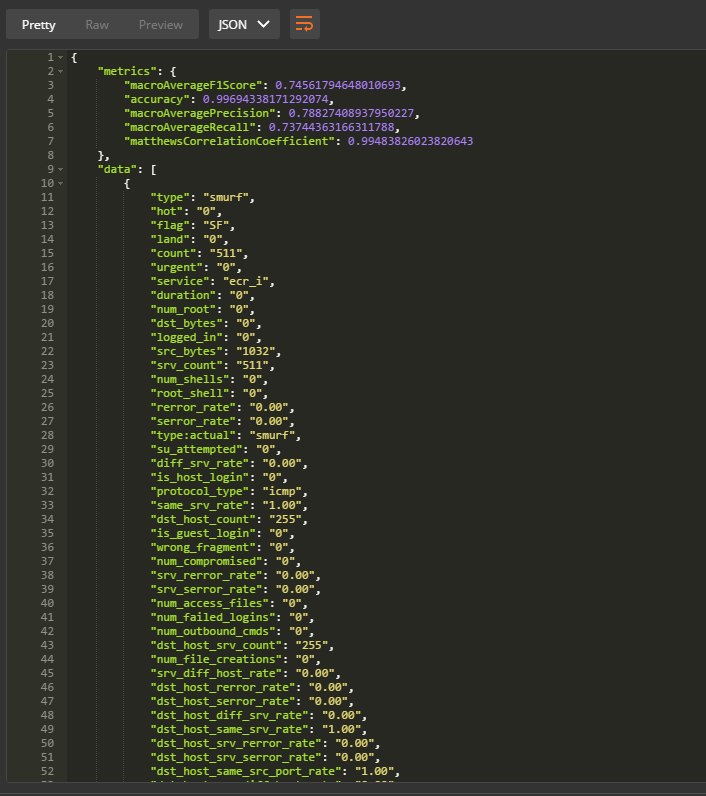
Understanding the Results
The metrics returned in the session results as follows:
{
    "metrics": {
        "macroAverageF1Score": 0.74561794648010693,
        "accuracy": 0.99694338171292074,
        "macroAveragePrecision": 0.78827408937950227,
        "macroAverageRecall": 0.73744363166311788,
        "matthewsCorrelationCoefficient": 0.99483826023820643
    },
    "data": [ ... data elided ...]
    "pageNumber": 0,
    "totalPages": 1977,
    "pageSize": 50,
    "totalCount": 98802,
    "sessionId": "0161de6c-d28c-4e0f-84da-a07ed56aa750",
    "type": "model",
    "status": "completed",
    "predictionDomain": "classification",
    "availablePredictionIntervals": [],
    "modelId": "d0f17138-eb6f-4b38-a41d-cc1c1d672436",
    "requestedDate": "2018-02-12T21:51:27.731942+00:00",
    "statusHistory": [
        {
            "date": "2018-02-12T21:51:27.731942+00:00",
            "status": "requested"
        },
        {
            "date": "2018-02-12T21:51:28.1771348+00:00",
            "status": "started"
        },
        {
            "date": "2018-02-12T22:40:16.3590024+00:00",
            "status": "completed"
        }
    ],
    "extraParameters": {
        "balance": true
    },
    "messages": [
        {
            "severity": "warning",
            "message": "Target class 'phf' is only specified on 4 record(s) in the dataset. Nexosis requires a minimum of 5 records per class for the class to be included in a model. Therefore, the model we generate will not consider this class."
        },
        {
            "severity": "warning",
            "message": "Target class 'spy' is only specified on 2 record(s) in the dataset. Nexosis requires a minimum of 5 records per class for the class to be included in a model. Therefore, the model we generate will not consider this class."
        },
        {
            "severity": "warning",
            "message": "Target class 'perl' is only specified on 3 record(s) in the dataset. Nexosis requires a minimum of 5 records per class for the class to be included in a model. Therefore, the model we generate will not consider this class."
        },
        {
            "severity": "informational",
            "message": "494011 observations were found in the dataset."
        }
    ],
    "name": "predictAttackType",
    "dataSourceName": "kddcup-training",
    "dataSetName": "kddcup-training",
    "targetColumn": "type",
    "algorithm": {
        "name": "Random Forest",
        "description": "Random Forest",
        "key": ""
    },
    "isEstimate": false,
    "links": [
        {
            "rel": "self",
            "href": "https://ml.nexosis.com/v1/sessions/0161de6c-d28c-4e0f-84da-a07ed56aa750/results"
        },
        {
            "rel": "model",
            "href": "https://ml.nexosis.com/v1/models/d0f17138-eb6f-4b38-a41d-cc1c1d672436"
        },
        {
            "rel": "confusionMatrix",
            "href": "https://ml.nexosis.com/v1/sessions/0161de6c-d28c-4e0f-84da-a07ed56aa750/results/confusionmatrix"
        },
        {
            "rel": "featureImportance",
            "href": "https://ml.nexosis.com/v1/sessions/0161de6c-d28c-4e0f-84da-a07ed56aa750/results/featureimportance"
        },
        {
            "rel": "classScores",
            "href": "https://ml.nexosis.com/v1/sessions/0161de6c-d28c-4e0f-84da-a07ed56aa750/results/classScores"
        },
        {
            "rel": "contest",
            "href": "https://ml.nexosis.com/v1/sessions/0161de6c-d28c-4e0f-84da-a07ed56aa750/contest"
        },
        {
            "rel": "first",
            "href": "https://ml.nexosis.com/v1/sessions/0161de6c-d28c-4e0f-84da-a07ed56aa750/results?page=0"
        },
        {
            "rel": "next",
            "href": "https://ml.nexosis.com/v1/sessions/0161de6c-d28c-4e0f-84da-a07ed56aa750/results?page=1"
        },
        {
            "rel": "last",
            "href": "https://ml.nexosis.com/v1/sessions/0161de6c-d28c-4e0f-84da-a07ed56aa750/results?page=1976"
        },
        {
            "rel": "vocabularies",
            "href": "https://ml.nexosis.com/v1/vocabulary?createdFromSessionid=0161de6c-d28c-4e0f-84da-a07ed56aa750"
        }
    ]
}
macroAverageF1Score- A measure of a tests accuracy considering both precision and recall of the tests.accuracy- The statistical measure of the proportion of true results (true positives and true negaties) over the total number of items.precision- true positives per predicted positiverecall- true positives per real positive
Accuracy
The accuracy metric reads 0.99694338171292074 - which can be converted to a percent by multiplying by 100 and rounding. The accuracy of this model is ~99.7%, meaning that when Nexosis analyzed the test set against the model, 99%.7% of the predictions made by the model were correct.
Now before we go and conclude this seemingly almost perfect model, it’s important to explore other information about the model’s performance since this one accuracy metric does not tell the entire story.
Macro Average F-Score
The macroAverageF1Score metric is another very important metric to look at in a multi-class classification model. It demonstraites how well the model performs overall across all the classes in the dataset. A macro-average computes the accuracy independently for each specifc class type and then take the harmonic mean - the important take-away of this metric is that it treats all classes equally, where-as the overall accuracy metric does not and thus may give you a false sense of the models ability to predict well for each and every class. The F1 score will be between 0 and 1 - closer to one is better.
“In computer science, specifically information retrieval and machine learning, the harmonic mean of the precision (true positives per predicted positive) and the recall (true positives per real positive) is often used as an aggregated performance score for the evaluation of algorithms and systems: the F-score (or F-measure).”
Source: Wikipedia
For our model, the macroAverageF1Score reads 0.74561794648010693, we can round to ~0.75. A score of 1 would be perfect, and ~0.75 is decent, but not stellar.
Confusion Matrix
A way to visualize understand how well a model is working is to get the confusion matrix - this, along with the metrics described above can give us a more complete picture of how the model is performing.
- From the Nexosis API Collection, open the Sessions folder and click
GET Retrieve Confusion Matrix (by SessionId)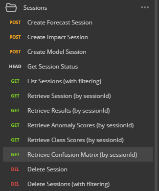 If you don’t have the Nexosis API collections, you can simply select GET from the dropdown and type https://ml.nexosis.com/v1/sessions/:sessionId/results/confusionmatrix in the text bar.

- Click Params and paste the unique session ID for sessionId Value.
Note: Your session ID can be found on the previous Postman tab. For this example, the
sessionIdis0161de6c-d28c-4e0f-84da-a07ed56aa750. - Click the blue
Sendbutton to the Right of the URL in Postman.

- The list of classes and then the confusion matrix results.
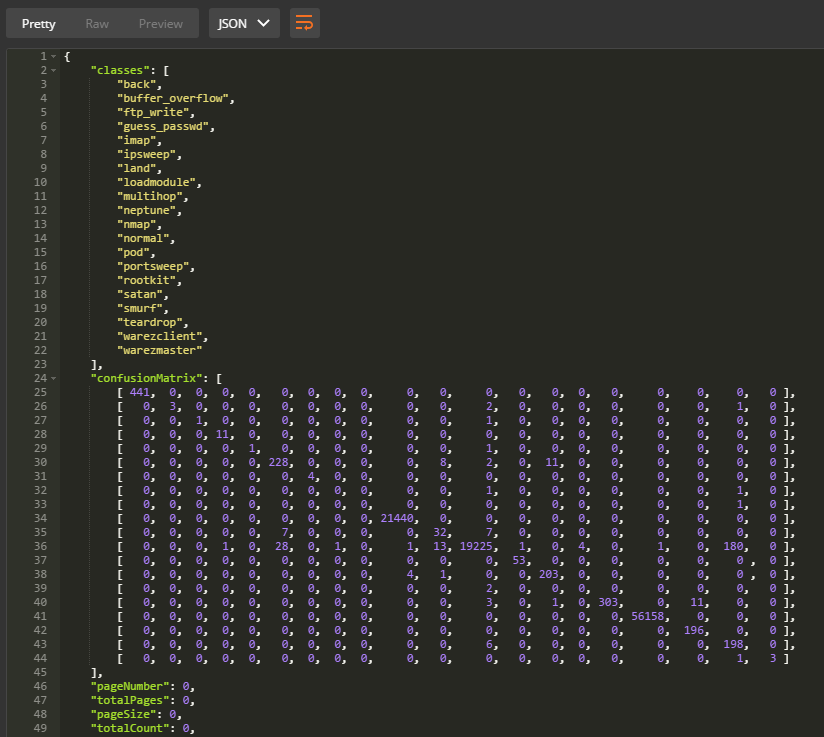
- Taking the JSON response, it’s trivial to draw the confusion matrix to make it more readable like so:
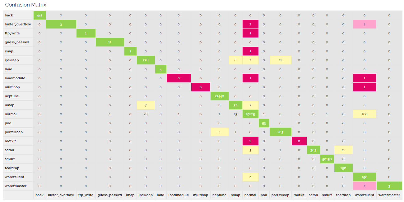
This confusion matrix shows the following:
- Actual class values are shown down the left side.
- Predicted class values are shown across the bottom.
- If prediction matches the actual, they will tally along the diagnal where the actual values intersect with the correct predictions.
- A good model should have most of the values tallied up along the diagnal.
- Any predictions that did not match the actual are tallied where the actual and the prediction intersect, off diagnal.
Conclusions
- Data labeled
normalis heavily represented in the dataset. - Data labeled
normalis rarely incorrectly classified as attack traffic. - When building the model, since we did not specify the
extraParametersand set thebalance, it will default totrue. This will then weight the under-represented classes so they are better represented by the model. - These classes did not predict well, potentially due to being unrepresented in the training set:
loadmodulemultihoprootkitbuffer_overflowftp_writeimap
- These classes performed well, though many of these classes did not have very many rows to train:
backguess_passwdipsweeplandneptunenormalpodportsweepsatansmurfteardropwarezclientwarezmaster
Given the grid above, we can conclude our model is likely really good at predicting some types of network attacks and mediocre to terrible on other classes.
Read More on our Blog by reading What is a Confusion Matrix and Classification Scoring Metrics for more details.
Next steps
Overall, this first experiment attempting to classifying attack traffic went decently well. With some basic data wrangling we built a model that had a high overall accuracy, but learned that’s only part of the story. We concluded from the Confusion Matrix and F-score that our model is really good at predicting some classes and not so great at others. Depending on our needs, this model might be useful as-is, but we intentionally skipped one important step. The KDD Cup challenge wanted only 5 categories of network attacks classified, not 20!
In the next part of this tutorial, we’ll start with the existing kddcup-training.csv CSV and add a new column called attack_class. It will compute a new column using the mapping defined by the KDD Cup 99 shown in Table 3 above to include five general attack categories. Additionally, we’ll add one more column while we’re at it that just has two categories called is_attack - this model can be used to identify normal traffic vs attack traffic.
Finally, we’ll explore the full large dataset to see if there is more data of the under-represented attack classes to include in training to further improve the model.
The goal of the experimentation is to see if it’s possible to increase the F-score.

