Classification
Forecasting
Impact of Television on Bigfoot Sightings
This tutorial will use JavaScript and the Nexosis API to explore the impact of television on bigfoot sightings
We’ll be doing this using JavaScript and the JavaScript Nexosis API client. I’m assuming that you know JavaScript, ES6, and Node.js. We will be using many of the built in array functions and ES6 Promises. We’ll also be using Moment.js since it makes working with dates in JavaScript much much easier.
The full source code is on GitHub. I won’t be showing all the code in this tutorial, just the interesting parts, so go ahead and clone it now so you can follow along.
My hypothesis is that the airing of popular television shows featuring bigfoot and other similar cryptids should result in an increase of the number of bigfoot sightings.
I have selected two shows to test my hypothesis:
- The X-Files which aired September 1993 through May 2002
- The Six Million Dollar Man which had several episodes in 1976 and 1977 featuring bigfoot

The big challenge here is where to get the data.
Fortunately, there is an organization that tracks sasquatch sightings. They call themselves the Bigfoot Field Researchers Organization or BFRO and they have detailed reports going back to the late 19th century. These reports include dates, locations, and even a classification of the sighting. All of the reports are available online.
The Internet has everything.
Of course, the reports aren’t in a very useful format. They are mostly unstructured data written by humans for humans to consume. Simple web pages that aren/t very machine friendly. But Timothy Renner loves weird data and he screen-scraped the entire dataset and published it to data.world. There, he has a CSV file with almost 4,000 geocoded sightings containing the date of the sighting, the classification, and the latitude and longitude of the sighting.
The Internet never ceases to amaze me.
So, armed with this data let’s set out to test my hypothesis.
The Raw Data
If we look inside bfro-report-locations.csv we’ll see it looks like this:
number,title,classification,timestamp,latitude,longitude
637,Report 637: Campers' encounter just after dark in the Wrangell - St. Elias National Park and Preserve,Class A,2000-06-16T12:00:00Z,61.5,-142.9
2917,Report 2917: Family observes large biped from car,Class A,1995-05-15T12:00:00Z,55.1872,-132.7982
7963,Report 7963: Sasquatch walks past window of house at night,Class A,2004-02-09T12:00:00Z,55.2035,-132.8202
9317,"Report 9317: Driver on Alcan Highway has noon, road encounter near Alaska-Canada border",Class A,2004-06-18T12:00:00Z,62.9375,-141.5667
13038,"Report 13038: Snowmobiler has encounter in deep snow near Potter, AK",Class A,2004-02-15T12:00:00Z,61.0595,-149.7853
...
This is the data we have. But, it’s not exactly how we’d like it to be. In fact, since we only care about number of sightings, most of it is not useful at all to our problem. There are two bits that we care about:
- Row existence If there is a row then exactly one sighting occurred.
- The timestamp This tells us when the sighting occurred.
Sightings can occur on the same day so we’ll need to aggregate those events before we update it to the Nexosis API. And since we’re aggregating, we might as well count up the empty days as well. Normally, you could use our API to do this automatically but I’d like to be able to generate a graph showing the number of bigfoot sightings over a period of time so I can visually compare it the impact analyses we are going to do.
And while we at it, let’s go ahead and aggregate the data monthly since we have many years worth of data and this will make it a little easier to work with when we generate our charts using Google Sheets.
There are also a few stray and sparse events that I’d like to prune out since it makes the chart hard to read. There’s even a bogus event talking about a sighting in 2053 during a Girl Scout campout. So, we’ll filter out any record before 1950 and any record after 2016. This will be plenty for us to see the impacts of 20th-century television shows.
Aggregating the Data
All the code for aggregating the data can be found in aggregate.js. To run
this code, enter the following command:
$ npm run aggregate
You can also call this with the following command line arguments:
| Argument | Description | Default |
|---|---|---|
| –startDate | start date in format YYYY-MM | 1950-01 |
| –endDate | end date in format YYYY-MM | 2017-01 |
| –input | path to input file | bfro-report-locations.csv |
| –output | path to output file | data/monthly-bigfoot-sightings.csv |
$ npm run aggregate -- --startDate=1975-01 --endDate=2000-12 --input=foo.csv --ouput=bar.csv
The relevant code for all this argument parsing is at the top of aggregate.js
and makes use of a node package called yargs. It’s super-easy to use as you can
see here.
const argv = require('yargs').argv

const INPUT_FILE = argv.input || 'bfro-report-locations.csv';
const OUTPUT_FILE = argv.output || 'data/monthly-bigfoot-sightings.csv';
const START_DATE = argv.startDate || '1950-01';
const END_DATE = argv.endDate || '2017-01';
After the argument parsing, there is the main promise chain. This is interesting because it controls the overall process of aggregating the data. I like it because it reads like a series of steps, which, it pretty much is.
loadRawSightings(INPUT_FILE)
  .then(sightings => transformSightings(sightings))
  .then(transformedSightings => aggregateSightings(transformedSightings))
  .then(aggregatedSightings => saveMontlySightings(aggregatedSightings, OUTPUT_FILE))
  .then(() => console.log('Aggregation completed!'));
Step one is to load the sightings from the raw CSV input file. The csvtojson
package does this and, living up to its name, loads the CSV file and makes it
JSON. This JSON matches the CSV structure.
const CSV = require('csvtojson');

function loadRawSightings(filename) {
  console.log(`Loading raw data from ${filename}...`);
  return new Promise(function(resolve, reject) {
    let sightings = [];
    CSV()
      .fromFile(filename)
      .on('json', sighting => sightings.push(sighting))
      .on('done', () => resolve(sightings));
  });
}
This structure is then transformed into data we care about, namely dates and quantities. Note that the quantity is always 1 and the date consists of just the year and month. Moment.js will will treat this as the first of the month. Since we are aggregating monthly, this is all will really want. Plus, it makes the aggregation easier in the next step.
const moment = require('moment');

function transformSightings(sightings) {

  console.log(`Transforming ${sightings.length} sightings...`);

  return sightings
    .map(sighting => transformSighting(sighting));

  function transformSighting(sighting) {
    return {
      date: justTheYearAndMonth(sighting.timestamp),
      quantity: 1
    }
  }

  function justTheYearAndMonth(dateTime) {
    return moment(dateTime.substring(0,7));
  }
}
Aggregating the sightings is a two-step process. First, we need to get all the months that we care about. The code that does this is not terribly inspired so I have not included it. Once we have an array of those months we can map them to an array of objects that contain the date and the quantity. This is the data we need to do our impact analyses.
Computing the quantity is interesting as we first use .filter to filter out
the sightings where the dates don’t match. Then, we use .reduce to add up the
quantities in each of the remaining sightings.
function aggregateSightings(sightings) {

  let months = generateMonthlyDateRanges();

  console.log(`Aggregating ${sightings.length} sightings to ${months.length} months...`);

  return months
    .map(date => aggregateSightingsForMonth(date));

  function aggregateSightingsForMonth(date) {
    let quantity = countSightingsForMonth(date);
    return { date, quantity };
  }

  function countSightingsForMonth(date) {
    return sightings
      .filter(sighting => sighting.date.isSame(date))
      .reduce((accumulator, sighting) => accumulator + sighting.quantity, 0);
  }
}
The final step is to save the new JSON data back out to CSV in a Google Sheets
friendly format. The formatting is handle by a quick transformation of the data
using .map and then we save the file using csv2json and the basic file system
methods that are a part of Node.js.
const json2csv = require('json2csv');
const fs = require('fs');
const moment = require('moment');

function saveMontlySightings(sightings, filename) {

  console.log(`Saving aggregated sightings to ${filename}...`);

  formattedSightings = sightings.map(sighting => formatSighting(sighting));
  return saveToCSV(formattedSightings, filename, );

  function formatSighting(sighting) {
    return {
      date: sighting.date.format('M/D/YYYY'),
      quantity: sighting.quantity
    }
  }

  function saveToCSV(data, filename) {
    let csv = json2csv({ data, fields: ['date', 'quantity'] });
    return saveToFile(csv, filename);
  }

  function saveToFile(data, filename) {
    return new Promise(function(resolve, reject) {
      fs.writeFile(filename, data, err => err ? reject(err) : resolve());
    });
  }
}
First Glance
So now we have a file that looks like this.
"date","quantity"
"1/1/1950",1
"2/1/1950",0
"3/1/1950",0
"4/1/1950",0
"5/1/1950",1
"6/1/1950",0
...
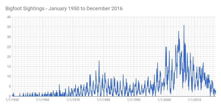
Let’s load this data up into a chart and see what it looks like.

Immediately two peaks show up. One in the late 70s and a significant rise in the 90s leading to a peak in 2007. These timeframes correlate to the shows we have selected.
Another interesting thing is observable here. Bigfoot sightings tend to occur in the middle of the calendar year and not at the beginning and end. That’s why we see all the spikes. This means that more sightings occur during the summer months than in the winter months. One might guess that bigfoot hibernates but my guess is that people don’t venture outside as often in the winter. There are not fewer bigfeet in the winter. There are fewer sightings.
Regardless of hibernation, our hypothesis is looking good already.
Uploading the Data
In order to do impact analyses on our data, we need to get it loaded. All the
code for uploading the data can be found in upload.js. To run this code,
enter the following command:
$ npm run upload
You can also call this with the following command line arguments:
| Argument | Description | Default |
|---|---|---|
| –input | path to input file | data/monthly-bigfoot-sightings.csv |
| –datasetName | name of the dataset to create | bigfootsightings |
| –apiKey | your Nexosis API key | value in NEXOSIS_API_KEY environment variable |
$ npm run upload -- --datasetName=biggerFoot --input=foo.csv --apiKey=YOUR_API_KEY
Once again we use yargs for this.
const argv = require('yargs').argv

const INPUT_FILE = argv.input || 'data/monthly-bigfoot-sightings.csv';
const DATASET_NAME = argv.datasetName || 'bigfootsightings';
const NEXOSIS_API_KEY = argv.apiKey || process.env.NEXOSIS_API_KEY;
So how does the upload work? Well, it starts with a promise chain just like
in aggregate.js.
removeExistingDataset(DATASET_NAME)
  .then(() => loadAggregatedSightings(INPUT_FILE))
  .then(sightings => transformSightings(sightings))
  .then(transformedSightings => uploadSightings(transformedSightings, DATASET_NAME))
  .then(() => console.log('Upload complete!'));
First, if there is a dataset with the same name, we remove it. Odds are, you’ll want to run this many times. If you do, it’s best to clean everything out first. If there are existing events with the same date, they will be overwritten. But any events that aren’t overwritten will stick around. We don’t want that.
We remove our dataset by using the Nexosis client to get a list of all the
datasets and finding out if it exists using the .some function on array. If
it does, we remove it.
const NexosisClient = require('nexosis-api-client').default
const client = new NexosisClient({ key: NEXOSIS_API_KEY });

function removeExistingDataset(datasetName) {
  return client.DataSets.list()
    .then(datasets => isDatasetAlreadyLoaded(datasets))
    .then(isLoaded => deleteIfLoaded(isLoaded));

  function isDatasetAlreadyLoaded(datasets) {
    console.log(`Looking for existing dataset ${datasetName}...`);
    return datasets.items.some(item => item.dataSetName === datasetName);
  }

  function deleteIfLoaded(isLoaded) {
    if (isLoaded) {
      console.log('Dataset was found. Removing...');
      return client.DataSets.remove(datasetName);
    } else {
      console.log('Dataset was not found. Continuing...');
    }
  }
}
Now that we have a clean slate, let’s load up the monthly sightings. We’ll do this with csvtojson just like we did when we loaded the raw CSV data during aggregation.
const CSV = require('csvtojson');

function loadAggregatedSightings(filename) {
  console.log(`Loading aggregated data from ${filename}...`);
  return new Promise(function(resolve, reject) {
    let sightings = [];
    CSV()
      .fromFile(filename)
      .on('json', sighting => sightings.push(sighting))
      .on('done', () => resolve(sightings));
  });
}
Once we have them loaded we need to convert the date to a valid ISO 8601 date
which, in this case, is YYYY-MM-DD. We’ll use .map and Moment.js to do that.
const moment = require('moment');

function transformSightings(sightings) {

  console.log(`Transforming ${sightings.length} months of sightings...`);

  return sightings
    .map(sighting => transformSighting(sighting));

  function transformSighting(sighting) {
    return {
      date: moment(sighting.date, 'M/D/YYYY').format('YYYY-MM-DD'),
      quantity: sighting.quantity
    };
  }
}
Now that our we have our data ready to upload, let’s upload it. Using the Nexosis
API Client for JavaScipt to do this is pretty easy. You just call .create with
all the data.
const NexosisClient = require('nexosis-api-client').default
const client = new NexosisClient({ key: NEXOSIS_API_KEY });

function uploadSightings(sightings, datasetName) {
  console.log(`Loading ${sightings.length} months of sightings...`);
  return client.DataSets.create(datasetName, { data: sightings });
}
And, our data is uploaded. If you’d like to confirm it you can use the following curl command.
$ curl -v -X GET "https://ml.nexosis.com/v1/data/bigfootsightings" -H "api-key: YOUR_API_KEY"
Which should return something like this:
{
  "dataSetName": "bigfootsightings",
  "columns": {
    "date": {
      "dataType": "date",
      "role": "timestamp"
    },
    "quantity": {
      "dataType": "numeric",
      "role": "target",
      "imputation": "zeroes",
      "aggregation": "sum"
    }
  },
  "data": [
    { "date": "1950-01-01", "quantity": "1" },
    { "date": "1950-02-01", "quantity": "0" },
    { "date": "1950-03-01", "quantity": "0" },
    { "date": "1950-04-01", "quantity": "0" },
    { "date": "1950-05-01", "quantity": "1" },
    { "date": "1950-06-01", "quantity": "0" },
      ...
  ],
  "links": [
    {
      "rel": "sessions",
      "href": "https://ml.nexosis.com/v1/sessions?dataSourceName=bigfootsightings"
    }
  ]
}
The Impact Analyses
Now we that we have our data loaded, let’s do some analysis. All the code for
impact analysis is can be found in impact.js. To run this code, enter the
following command:
$ npm run impact
You can also call this with the following command line arguments:
| Argument | Description | Default |
|---|---|---|
| –datasetName | name of the dataset to analyze | bigfootsightings |
| –output | path to output file | data/impact-on-bigfoot-sightings.csv |
| –metrics | path to metrics file | data/impact-on-bigfoot-sightings-metrics.csv |
| –startDate | start date for the impact period in format YYYY-MM | 1993-09 |
| –endDate | end date for the impact period in format YYYY-MM | 2002-05 |
| –eventName | the event name to be used for this impact analysis | impact-on-bigfoot-sightings |
| –apiKey | your Nexosis API key | value in NEXOSIS_API_KEY environment variable |
| –pollingInterval | how long to wait before checking if the analysis is completed in seconds | 60 |
$ npm run impact -- --datasetName=biggerFoot --output=foo.csv --apiKey=YOUR_API_KEY
And yet again we use yargs for this.
const argv = require('yargs').argv

const DATASET_NAME = argv.datasetName || 'bigfootsightings';
const OUTPUT_FILE = argv.output || 'data/impact-on-bigfoot-sightings.csv';
const METRICS_FILE = argv.metrics || 'data/impact-on-bigfoot-sightings-metrics.csv';
const START_DATE = argv.startDate || '1993-09';
const END_DATE = argv.endDate || '2002-05';
const EVENT_NAME = argv.eventName || 'impact-on-bigfoot-sightings';
const NEXOSIS_API_KEY = argv.apiKey || process.env.NEXOSIS_API_KEY;
const POLLING_INTERVAL = (Number(argv.pollingInterval) || 60) * 1000;
This code also starts with a promise chain. Note the call to Promise.all that
saves the data and metrics in parallel. Neat!
createImpactAnalysis(DATASET_NAME, START_DATE, END_DATE, EVENT_NAME)
  .then(session => fetchResults(session.sessionId, POLLING_INTERVAL))
  .then(results => Promise.all([
    saveImpactData(results.data, OUTPUT_FILE),
    saveImpactMetrics(results.metrics, METRICS_FILE)
  ]))
  .then(() => console.log("Impact Analysis completed!"));
The chain starts out with a request to begin the impact analysis. This code is really straightforward. Just use the client to start the session and return the promise.
const NexosisClient = require('nexosis-api-client').default
const client = new NexosisClient({ key: NEXOSIS_API_KEY });

function createImpactAnalysis(datasetName, startDate, endDate, eventName) {
  console.log(`Creating impact session on dataset ${datasetName} for time period ${startDate} through ${endDate}...`)
  return client.Sessions
    .analyzeImpact(datasetName, startDate, endDate, eventName, 'quantity', 'month');
}
This promise will resolve to the session that was created. In there, we really only care about the session ID as we need it to check the session status and to retrieve the results.
Fetching the results is interesting and a little hairy since we need to poll the
API to check the status. We make a call to setInterval inside of a promise to
do this. Once the call to checkStatus completes with a status of either
completed, failed, or cancelled we know there is nothing left to do but
fetch the results (or the error) and resolve the promise.
const NexosisClient = require('nexosis-api-client').default
const client = new NexosisClient({ key: NEXOSIS_API_KEY });

function fetchResults(sessionId, interval) {
  console.log(`Fetching session results for impact session ${sessionId}`);

  return new Promise(function(resolve, reject) {
    let intervalHandle = setInterval(checkStatus, interval);

    function checkStatus() {
      console.log(`Checking status for impact session ${sessionId}`);

      fetchStatus().then(status => {
        if (isDone(status)) {
          clearInterval(intervalHandle);
          fetchResults()
        }
      })
    }

    function fetchStatus() {
      return client.Sessions.get(sessionId).then(session => session.status)
    }

    function isDone(status) {
      return ['completed', 'failed', 'cancelled'].includes(status);
    }

    function fetchResults() {
      return client.Sessions.results(sessionId)
        .then(results => resolve(results))
    }

  });
}
Now that we have the results we can save the impact data and the impact metrics. The data will show us how many bigfoot sightings we should have expected based on the history of sightings up until that point. The metrics will show us how much that deviated and the impact of it. We save the data and metrics to CSV files using json2csv and the Node.js file system features, just like we did during aggregation.
const json2csv = require('json2csv');
const fs = require('fs');
const moment = require('moment');

function saveImpactData(data, filename) {

  console.log(`Saving impact data to ${filename}...`);

  let formattedData = data
    .map(sighting => formatSighting(sighting));

  return saveToCSV(formattedData, filename, ['date', 'quantity']);

  function formatSighting(sighting) {
    return {
      date: moment(sighting.date).format('M/D/YYYY'),
      quantity: Number(sighting.quantity)
    }
  }
}

function saveImpactMetrics(metrics, filename) {
  console.log(`Saving impact metrics to ${filename}...`);
  return saveToCSV(metrics, filename, ['pValue', 'absoluteEffect', 'relativeEffect']);
}

function saveToCSV(data, filename, fields) {
  let csv = json2csv({ data, fields });
  return saveToFile(csv, filename);
}

function saveToFile(data, filename) {
  return new Promise(function(resolve, reject) {
    fs.writeFile(filename, data, err => err ? reject(err) : resolve());
  });
}
So now we have a functional tool to run impact analyses. Let’s run them!
The Six Million Dollar Man
First, The Six Million Dollar Man. My wife and I both have fond memories of watching this show as kids. I can hear the dated sound effect letting us know that Lee Majors was using his bionic enhancements as I type this. Ah, glorious nostalgia!
Lee Majors graced us with his bionic presence for five years from January of 1974 until March of 1978. Bigfoot did not make an appearance on the show until February of 1976. Let’s use that as the start date and the end of the series as the end date for our impact analysis.
Let’s run the command.
$ npm run impact -- --startDate=1976-02 --endDate=1978-03 --eventName=six-million-dollar-man \
                    --output=data/six-million-dollar-man-impact-data.csv \
                    --metrics=data/six-million-dollar-man-impact-metrics.csv \
                    --apiKey=YOUR_API_KEY
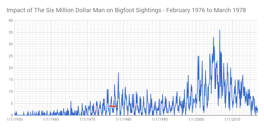
Loading this into Google Sheets so we can get some charts we see the predicted vs. actual results. This will give us a feel for the impact.

Hmmm… looks like there might be some impact. What do the metrics say? Looking at them we see the following:
| Metric | Value |
|---|---|
| p-value | 0.3374 |
| absolute effect | 6.5138 |
| relative effect | 0.0661 |
The p-value shows some correlation but not a very strong one. Certainly not below 0.05. It’s starting to look like The Six Million Dollar Man didn’t have a huge impact on bigfoot sightings. The general trend suggests that the number of sightings was increasing before the bigfoot episodes aired. Perhaps this is an example of art imitating life? Of course, there were only a handful of episodes related to the paranormal on The Six Million Dollar Man so maybe this is not so surprising.
Fun Fact #1
André the Giant played Bigfoot in Season 3, Episode 16 & 17 of The Six Million Dollar Man back in 1976. The episode was a two-parter called “The Secret of Bigfoot”. It was so popular they even made an action figure.

The X-Files
Now, let’s see how The X-Files stacks up. I started watching The X-Files shortly after graduating from college. I made sure I knew how to program my VCR so I could record the show and not miss an episode. I wanted to believe and I knew the truth was out there.
Mulder and Scully bickered about the existence of the paranormal from September 1993 through May 2002. Let’s determine the impact of the entire series run.
Here’s the command we need to run.
$ npm run impact -- --startDate=1993-09 --endDate=2002-05 --eventName=x-files \
                    --output=data/x-files-impact-data.csv \
                    --metrics=data/x-files-impact-metrics.csv \
                    --apiKey=YOUR_API_KEY
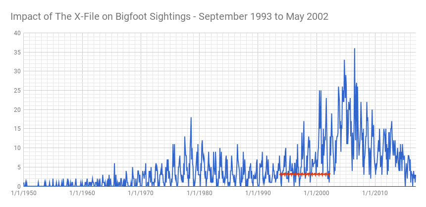
And generating a chart we see the following:

This seems a lot stronger than what we saw with The Six Million Dollar Man. The rise in bigfoot sightings carries on past the air dates of the show and into the mid-2000s. What do the metrics say?
| Metric | Value |
|---|---|
| p-value | 0.004 |
| absolute effect | 372.0222 |
| relative effect | 1.1173 |
These are much stronger numbers. I think we can confidently say that The X-Files impacted bigfoot sightings. Or… something. Perhaps life was imitating art?
Fun Fact #2
Surprisingly, bigfoot has never been featured on The X-Files. However, in Season 1, Episode 6 a sketch of the Jersey Devil distinctly resembles a very famous photograph of Bigfoot.

Extra Credit
With this data, you should be able to run some forecast sessions and predict how many bigfoot sightings we will see in 2017 and beyond. Try and figure that out using the examples in this tutorial. The implementation is in the repository but it’s more fun (and you’ll learn more) if you do it yourself.
Conclusions
This was, of course, all for fun. My actual hypothesis on the two spikes you see in the historical data in the 70s and later in the 90s are not that they are the result of television shows. While I did like both The Six Million Dollar Man and The X-Files I think they are unrelated. Particularly in the 90s and through the mid-2000s I believe the rise of the Internet increased the number of reported sightings without increasing the actual number of sightings. The radical level of communication the Internet brought has changed many things. I can’t really explain the spike in the 70s but the increase matches my memory of that decade. The 70s were a weird time.
Thanks for joining me in this journey. It’s been fun! I hope you’ve gotten a better understanding of how to use the Nexosis API with JavaScript from this tutorial and how you might be able to use forecasting and impact analysis to answer other (probably more important) questions.
